
Introduction: The Lifeblood of Optical Transmission
In the hyper-competitive landscape of B2B telecommunications, network reliability and transmission quality are non-negotiable. At the heart of every high-performance Dense Wavelength Division Multiplexing (DWDM) and long-haul network lies a critical, yet often misunderstood metric: Optical Signal to Noise Ratio (OSNR). As network architects and systems integrators push towards 800G and beyond, understanding OSNR isn’t just an engineering exercise—it’s the foundation of network ROI, service-level agreements (SLAs), and operational efficiency . This definitive guide provides a deep technical dive into OSNR, covering its architectural impact, measurement standards, and strategic deployment to ensure carrier-grade reliability.
Core Architecture: Understanding the Physics of OSNR
OSNR is the ratio of optical signal power to noise power within a specific effective bandwidth, typically 0.1 nm . It is the primary determinant of the Bit Error Rate (BER) before Forward Error Correction (FEC) intervenes . While simple in concept, the architecture of a network dictates how this ratio evolves.
The Dominant Noise Source: Amplified Spontaneous Emission (ASE)
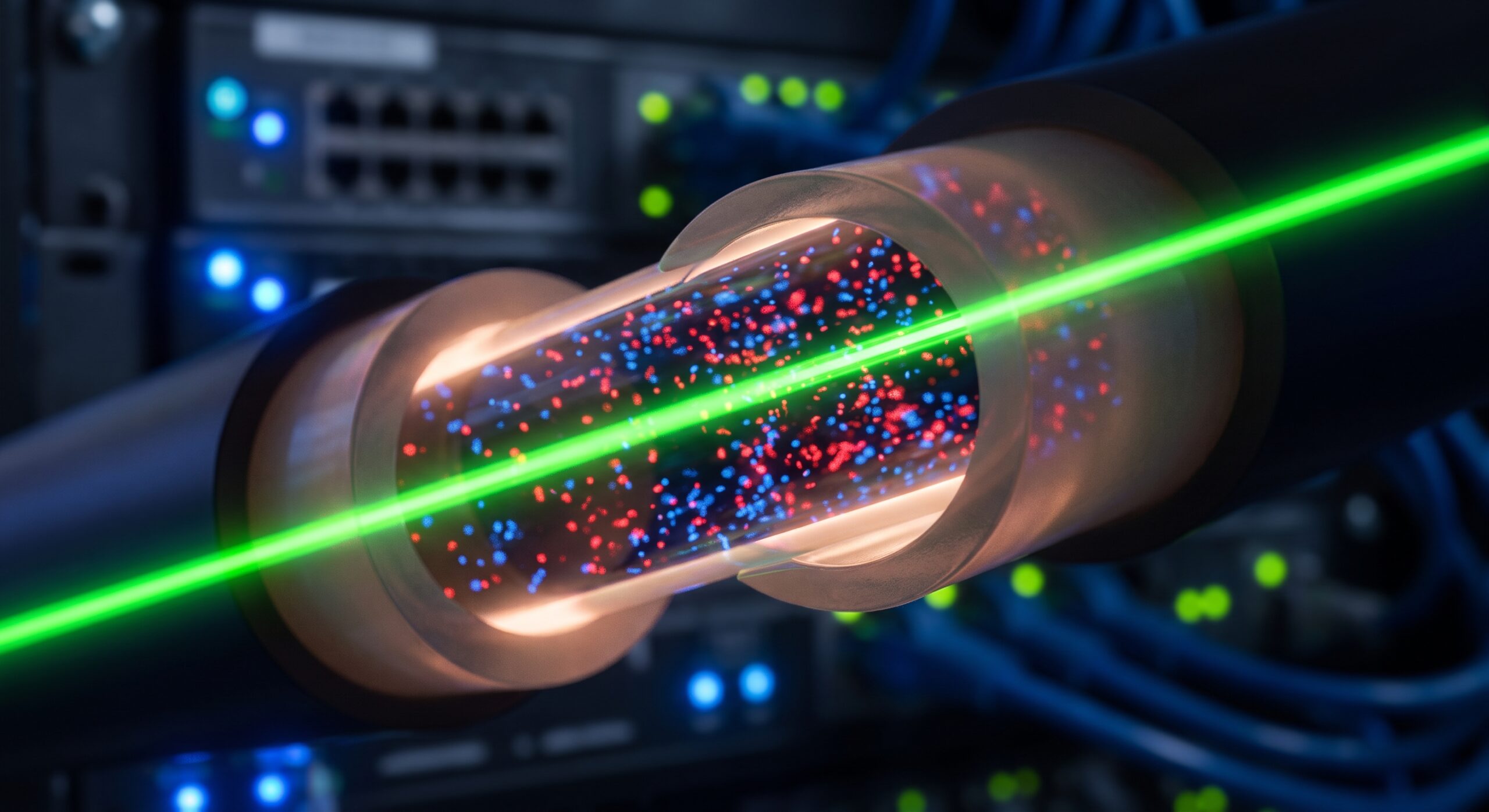
In long-haul systems, the primary contributor to noise is ASE, generated by optical amplifiers like Erbium-Doped Fiber Amplifiers (EDFAs) . Unlike traditional electrical repeaters, EDFAs amplify the optical signal directly but inevitably add noise through spontaneous emission. Each amplifier adds to the total noise floor, compounding the degradation of OSNR along the span. As a signal passes through an EDFA, the OSNR typically decreases by approximately 3 dB for the first amplifier, with subsequent additions degrading the ratio at a slower, yet compounding, rate .
The OSNR Formula and Evolution
For a single optical channel, the OSNR at the receiver can be expressed as a function of input power, amplifier gain (G), and noise figure (NF). The degradation per amplifier is heavily dependent on the amplifier’s NF; lower NF values result in higher output OSNR . The formula highlights the inverse relationship between noise accumulation and transmission distance—the farther the signal travels, the greater the ASE accumulation and the lower the OSNR.
| System Type | Modulation Format | Typical Required OSNR (dB) | Reference Standard | Key Limiting Factor |
|---|---|---|---|---|
| 10G Non-Coherent | OOK | 25+ (No FEC) | ITU-T G.957 | Linear ASE Noise |
| 100G Coherent | PM-QPSK | 15 – 18 | IEC 61280-2-9 / IEEE 802.3ba | ASE & Filtering |
| 200G/400G Coherent | PM-16QAM | 21 – 27+ | IEC 61282-12 / OpenZR+ | ASE & Non-Linear Effects |
| 800G Coherent | PM-64QAM / 128QAM | 30+ | C-Corridor 800G Specification | ASE & Phase Noise |
Technical Specifications: Benchmarks and Standards
Engineering a robust network requires strict adherence to industry specifications. OSNR requirements vary dramatically based on data rate and modulation format.
- Basic 10G Systems: Require an OSNR of approximately >25 dB without FEC .
- Coherent 100G/400G Systems: For modern PM-QPSK (100G) and PM-16QAM (200G/400G), the required OSNR threshold climbs significantly. A PM-QPSK system might have a B2B OSNR tolerance of around 15-18 dB, while higher-order modulations like 16QAM require 21-27 dB or more due to tighter constellation spacing .
- Modern Coherent DSP: While Digital Signal Processing (DSP) can compensate for chromatic dispersion and polarization mode dispersion, it cannot eliminate ASE noise. Maintaining sufficient OSNR remains the fundamental prerequisite for the receiver to lock onto the signal .
Standards Compliance: Measurement methods are standardized to ensure consistency. Traditional out-of-band measurements are defined under IEC 61280-2-9, while advanced in-band OSNR measurements, critical for ROADM-based networks and superchannels, are covered under IEC 61282-12 .
Deployment and Optimization: Strategies for Maximizing Performance
Effective network design involves not just calculating OSNR budgets but actively managing and optimizing them.
OSNR Balancing in High-Density DWDM
In multi-channel systems, different wavelengths experience varying power levels and amplifier gains, leading to OSNR discrepancies. OSNR Loss Balancing is an advanced technique used to adjust the gain profile across wavelengths, ensuring that the worst-performing channel meets the required threshold. This prevents a single “weak” channel from limiting the entire system’s transmission distance .
Advanced Amplification: The Raman Advantage
To extend transmission distances, engineers employ Raman amplifiers. Unlike EDFAs, Raman amplification provides distributed gain along the fiber itself, effectively reducing the noise figure of the overall amplification chain. This extends the reach of 10G and 40G signals significantly, allowing for longer spans and higher OSNR at the receiver .
Real-World Monitoring: The Role of the OSA
An Optical Spectrum Analyzer (OSA) is the primary tool for measuring OSNR. During activation, technicians use the OSA to check channel power and OSNR at the receiver. The data allows engineers to maximize the fiber’s potential by identifying if additional channels can be added to the spectrum or if an amplifier’s gain needs tuning. Advanced OSA capabilities are crucial for provisioning single-wave 800G systems .

Conclusion: The Imperative for OSNR Mastery
As network speeds scale to meet the demands of AI and cloud computing, the margin for error shrinks. OSNR is not merely a metric to be measured during commissioning; it is a continuous operational metric that dictates service quality and Mean Time Between Failures (MTBF). For B2B hardware providers and network architects, mastering OSNR architecture, adhering to stringent specs, and implementing advanced optimization techniques are non-negotiable for delivering high-performance, reliable, and future-proof telecom infrastructure. The future of data transmission is built on the clarity of the optical signal.
Leave a comment